
Statistical testing in null worlds
◎◉○
Learn the intuition behind p-values through simulation
There is only one test
At their core, all statistical tests† can be conducted by following a universal pattern:
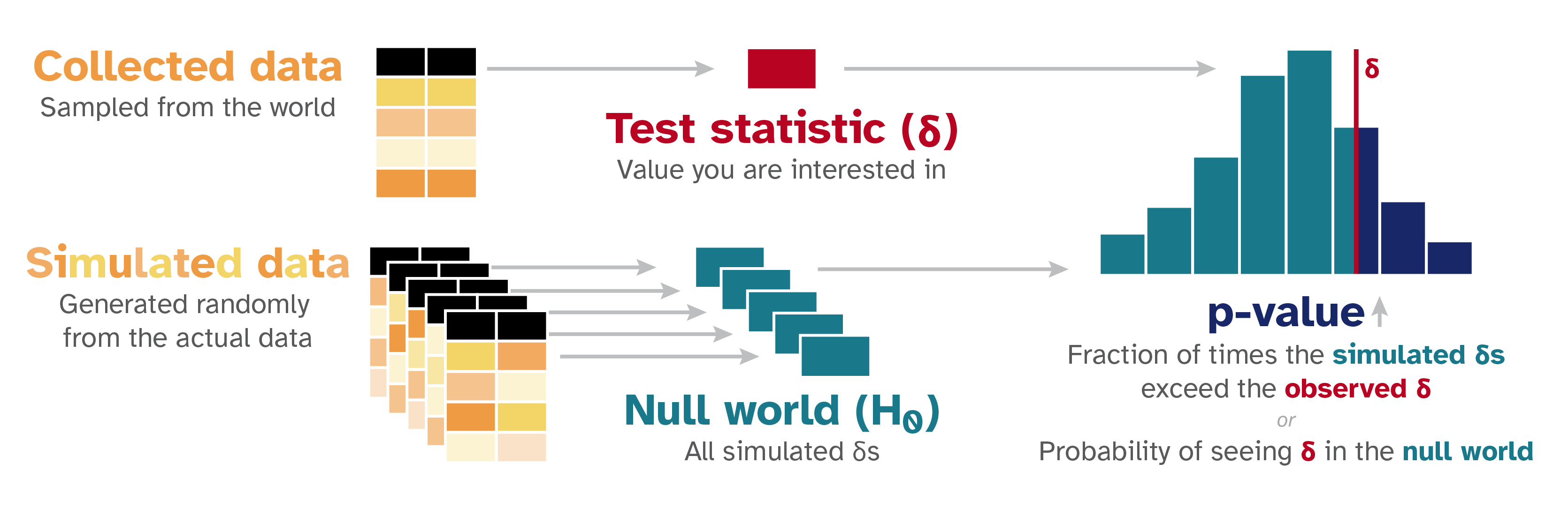
- Step 1: Calculate a sample statistic, or \(\delta\) (“delta”). This is the main measure you care about: the difference in means, the average, the median, the proportion, the difference in proportions, the slope in a regression model, an odds ratio, etc.
- Step 2: Use simulation to invent a world where \(\delta\) is null. Simulate what the world would look like if there was no difference or relationship between two groups, or if there was no difference in proportions, or where the average value is a specific number.
- Step 3: Look at \(\delta\) in the null world. Put the sample statistic in the null world and see if it fits well.
- Step 4: Calculate the probability that \(\delta\) could exist in the null world. This is the p-value, or the probability that you’d see a \(\delta\) at least as extreme in a world where there’s no difference.
- Step 5: Decide if \(\delta\) is statistically significant. Choose some evidentiary standard or threshold for deciding if there’s sufficient proof for rejecting the null world. Standard thresholds (from least to most rigorous) are 0.1, 0.05, and 0.01.
That’s all. Five steps. No need to follow complicated flowcharts to select the best and most appropriate statistical test. No need to decide which pretests you need to run to choose the right flavor of t-test. No need to think about whether you should use a t- or a z- distribution for your test statistic.
Simulate instead. There is only one test.
Calculate a number, simulate a null world, calculate the probability of seeing your number in that null world, and decide if that number is significantly different from what is typically seen in the null world.
Examples
This site contains a few different illustrations of common statistical tests:
Do I have to simulate everything?
No! In practice, you’ll typically run regular regressions, t-tests, or \(\chi^2\) tests. These use known theoretical distributions to approximate the null world mathematically rather than through simulation, but the intuition is identical: a p-value is still the probability of seeing a \(\delta\) at least as extreme in a world where there’s no difference.
Once you understand this general framework, “you can understand any hypothesis test”, even if it’s not done through simulation.
But simulation really shines when your \(\delta\) is something unusual—something that doesn’t have a convenient built-in test or a place in a statistical test flowchart.‡ Want to test a difference in group medians? Some interesting quantity that no textbook has ever named, like the average number of years a country ranks in the top five for GDP growth? You can test it! Define any \(\delta\) you want, simulate a null world for it, and get a valid p-value. No flowchart required. The {infer} package in R makes this straightforward.
For more examples of this process, and a more formal explanation of why it works, see Allen Downey’s “There is still only one test” and chapters 7–10 of ModernDive (especially chapter 8).
This all feels vaguely Bayesian?
Yep. All this simulation thinking is actually part of my clandestine plot to get more people curious about Bayesian statistics. This way of thinking prepares you for Bayesian inference, without actually being Bayesian.
This simulation-based approach mirrors a lot of the computational thinking behind Bayesian statistics. In both approaches, we (1) start with an explicit data-generating process and (2) think about uncertainty with simulation instead of formulas.
But there’s an important difference in what we’re simulating!
With traditional null hypothesis testing, we simulate a null world and ask:
If this were the world we lived in, how surprising would our observed \(\delta\) be?
Bayesian statistics flips this. Instead of asking how extreme our data (or \(\delta\)) is in a single null world, we model uncertainty about the parameter \(\delta\) itself. After combining prior beliefs with observed data, we get a posterior distribution that we can simulate from to ask:
What range of values of \(\delta\) are most plausible, given the data we’ve observed?
If that sounds fun—and if you’d rather say things like “there’s an X% probability that \(\delta\) is positive” or “\(\delta\) is most likely between X and Y” instead of the convoluted “in a world where \(\delta\) is 0ish, there’s an X% probability of seeing a \(\delta\) at least as extreme as what we observed”—check out Bayes Rules! for the best introduction I’ve found to Bayesian modeling.
Photo by BoliviaInteligente on Unsplash
Footnotes
At least for null hypothesis significance testing (NHST). Bayesian inference is different (see more about that below!). ↩︎
See chapter 1 of Richard McElreath’s Statistical Rethinking for more about issues with statistical test flowcharts. He has a free lecture video and slides and other resources here. ↩︎