One-sample mean

One-sample mean

◎◉○

Live simulation

jstat = require("jstat@1.9.6")

clrs = ({
  gold: "#f3d567",
  orange: "#ee9b43",
  coral: "#e74b47",
  crimson: "#b80422",
  navy: "#172767",
  teal: "#19798b",
  gray: "#4d4d4d"
})

function statLabel(value, textFn, dy, nullValues) {
  const extent = d3.extent([...nullValues, value]);
  const range = extent[1] - extent[0];
  const pos = range === 0 ? 0.5 :
    (value - extent[0]) / range;
  const textAnchor = pos > 0.82 ? "end" :
    pos < 0.18 ? "start" : "middle";
  const dx = textAnchor === "end" ? -10 :
    textAnchor === "start" ? 10 : 0;

  const common = {
    x: d => d, frameAnchor: "top", dy, dx,
    text: textFn,
    fontWeight: "bold", fontSize: 14,
    textAnchor, paintOrder: "stroke"
  };

  return [
    Plot.text([value], {
      ...common,
      stroke: "white", strokeWidth: 4, fill: "black"
    })
  ];
}

viewof sample_size = Inputs.range([30, 2000], {
  step: 10,
  value: 100,
  label: "Sample size:"
})

viewof comparison_value = Inputs.range([20, 80], {
  step: 1,
  value: 40,
  label: "Comparison value (μ₀):"
})

viewof effect_size = Inputs.range([-10, 10], {
  step: 1,
  value: 5,
  label: "Difference from μ₀:"
})

viewof spread = Inputs.range([1, 30], {
  step: 1,
  value: 10,
  label: "Spread (σ):"
})

sample_data = {
  const data = [];
  for (let i = 0; i < sample_size; i++) {
    data.push({
      outcome: jstat.normal.sample(
        comparison_value + effect_size, spread
      )
    });
  }
  return data;
}

Plot.plot({
  style: { fontSize: "13px" },
  marginLeft: 50,
  height: 250,
  x: { label: "Outcome" },
  y: { label: null },
  marks: [
    Plot.rectY(
      sample_data,
      Plot.binX(
        { y: "count" },
        {
          x: "outcome",
          fill: clrs.navy,
          thresholds: 20
        }
      )
    ),
    Plot.ruleX([comparison_value], {
      stroke: clrs.crimson,
      strokeWidth: 2.5,
      strokeDasharray: "6,3"
    }),
    Plot.text([comparison_value], {
      x: d => d,
      frameAnchor: "top",
      dy: 12,
      text: d => `μ₀ = ${d}`,
      fill: clrs.crimson,
      fontWeight: "bold",
      fontSize: 14,
      stroke: "rgba(255,255,255,0.7)",
      strokeWidth: 5,
      paintOrder: "stroke"
    }),
    Plot.ruleY([0])
  ]
})

Step 1: Calculate δ

The sample statistic (δ) is the difference between the sample mean and the comparison value (μ₀).

sample_stats = {
  const values = sample_data.map(d => d.outcome);
  const sample_mean = d3.mean(values);
  const se = d3.deviation(values) / Math.sqrt(values.length);
  const ci = [sample_mean - 1.96 * se, sample_mean + 1.96 * se];
  const delta = sample_mean - comparison_value;

  return { sample_mean, se, ci, delta, n: values.length };
}

obs_stat = sample_stats.sample_mean
delta = sample_stats.delta

html`<p>The sample mean is <strong>${sample_stats.sample_mean.toFixed(2)}</strong> and the comparison value is <strong>${comparison_value}</strong>, so δ = <strong>${delta.toFixed(2)}</strong>.</p>`

html`<table class="table table-sm" style="max-width: 500px;">
  <thead>
    <tr>
      <th></th>
      <th>Value</th>
      <th>95% CI</th>
    </tr>
  </thead>
  <tbody>
    <tr style="background-color: ${clrs.navy}11;">
      <td>Sample mean</td>
      <td>${sample_stats.sample_mean.toFixed(2)}</td>
      <td>[${sample_stats.ci[0].toFixed(2)}, ${sample_stats.ci[1].toFixed(2)}]</td>
    </tr>
    <tr style="background-color: ${clrs.orange}22;">
      <td>Comparison value (μ₀)</td>
      <td>${comparison_value.toFixed(2)}</td>
      <td></td>
    </tr>
    <tr style="background-color: ${clrs.crimson}; color: white; font-weight: bold;">
      <td>Difference (δ)</td>
      <td>${delta.toFixed(2)}</td>
      <td></td>
    </tr>
  </tbody>
</table>`

Step 2: Simulate null world

We create a null distribution by recentering and bootstrapping. We shift our data so its average equals the comparison value (μ₀), then resample from that shifted data (with replacement) hundreds of times. This creates a world where the population mean is the comparison value.

Think of this as being a world where the true mean is μ₀. Importantly, this doesn’t mean that every bootstrapped sample mean will be exactly μ₀. There is variation in the data, and that variation is reflected in the null world. What it means is that in the null world, the sample mean is μ₀ ± some amount.

Here’s what the recentering and resampling looks like. The left table shows the original data shifted so its mean equals μ₀. The right table shows one bootstrap resample drawn from that shifted data (with replacement—notice some rows appear more than once):

viewof resample = Inputs.button("Resample")

bootstrap_preview = {
  resample;
  const values = sample_data.map(d => d.outcome);
  const sample_mean = d3.mean(values);
  const shift = comparison_value - sample_mean;
  const centered = values.map(v => v + shift);
  const subset = centered.slice(0, 8);
  const n = subset.length;

  // Bootstrap resample from the subset
  const resampled = [];
  for (let i = 0; i < n; i++) {
    resampled.push(subset[Math.floor(Math.random() * n)]);
  }

  return {
    centered: subset.map((v, i) => ({
      " ": i + 1,
      Value: +v.toFixed(1)
    })),
    resampled: resampled.map((v, i) => ({
      " ": i + 1,
      Value: +v.toFixed(1)
    }))
  };
}

Recentered data

Inputs.table(bootstrap_preview.centered, {
  columns: [" ", "Value"],
  rows: 12,
  sort: false,
  select: false
})

Bootstrap resample

Inputs.table(bootstrap_preview.resampled, {
  columns: [" ", "Value"],
  rows: 12,
  sort: false,
  select: false
})

When we do this resampling hundreds of times and compute the mean each time, we get a null distribution—a picture of what sample means look like in a world where the true mean is μ₀.

Here’s what this null world looks like:

viewof n_reps = Inputs.range([100, 2000], {
  step: 100,
  value: 500,
  label: "Number of simulations:"
})

null_dist = {
  // Recenter data around comparison value
  const values = sample_data.map(d => d.outcome);
  const sample_mean = d3.mean(values);
  const shift = comparison_value - sample_mean;
  const centered = values.map(v => v + shift);

  const n = centered.length;
  const results = [];

  for (let r = 0; r < n_reps; r++) {
    // Bootstrap: sample with replacement
    let sum = 0;
    for (let i = 0; i < n; i++) {
      sum += centered[Math.floor(Math.random() * n)];
    }
    results.push({ stat: sum / n });
  }
  return results;
}

Plot.plot({
  style: { fontSize: "13px" },
  height: 300,
  width: 500,
  x: { label: "Bootstrapped mean" },
  y: { label: "Count" },
  marks: [
    Plot.rectY(
      null_dist,
      Plot.binX(
        { y: "count" },
        { x: "stat", fill: clrs.gray }
      )
    )
  ]
})

Step 3: Put δ in the null world

Next we put our observed sample mean inside that null world and see how comfortably it fits there.

Is it surprising to see the red line in this null world? Is the line way out to one of the sides, or is it near the middle with the rest of the null world?

Plot.plot({
  style: { fontSize: "13px" },
  height: 300,
  width: 500,
  x: { label: "Sample mean" },
  y: { label: "Count" },
  marks: [
    Plot.rectY(
      null_dist,
      Plot.binX(
        { y: "count" },
        { x: "stat", fill: clrs.gray }
      )
    ),
    Plot.ruleX([obs_stat], { stroke: "red", strokeWidth: 3 }),
    ...statLabel(obs_stat, d => `x̄ = ${d.toFixed(2)}`, 20,
      null_dist.map(d => d.stat))
  ]
})

Step 4: p-value

We can actually quantify the probability of seeing that red line in a null world. This is a p-value—the probability of seeing a sample mean at least that far from μ₀ in a world where the true mean is μ₀.

p_value = {
  const abs_dist = Math.abs(obs_stat - comparison_value);
  const extreme = null_dist.filter(
    d => Math.abs(d.stat - comparison_value) >= abs_dist
  ).length;
  return extreme / null_dist.length;
}

p_value_clean = p_value === 0
  ? "< 0.001"
  : p_value.toFixed(3)

p_percent = p_value === 0
  ? "< 0.1%"
  : (p_value * 100).toFixed(1) + "%"

null_bins = {
  const values = null_dist.map(d => d.stat);
  const bin = d3.bin().thresholds(30);
  const bins = bin(values);
  const abs_dist = Math.abs(obs_stat - comparison_value);
  return bins.map(b => ({
    x0: b.x0,
    x1: b.x1,
    count: b.length,
    extreme: Math.abs(((b.x0 + b.x1) / 2) - comparison_value)
      >= abs_dist
  }));
}

Plot.plot({
  style: { fontSize: "13px" },
  height: 300,
  width: 500,
  x: { label: "Sample mean" },
  y: { label: "Count" },
  marks: [
    Plot.rectY(null_bins, {
      x1: "x0",
      x2: "x1",
      y: "count",
      fill: d => d.extreme ? clrs.coral + "aa" : clrs.gray,
      stroke: "white",
      strokeWidth: 0.5
    }),
    Plot.ruleX([obs_stat], { stroke: "red", strokeWidth: 3 }),
    ...statLabel(obs_stat, d => `x̄ = ${d.toFixed(2)}`, 20,
      null_dist.map(d => d.stat)),
    ...statLabel(obs_stat, () => `p = ${p_value_clean}`, 45,
      null_dist.map(d => d.stat))
  ]
})

The p-value is

html`<p>This means that in a world where the true mean is <strong>${comparison_value}</strong>, there is a <strong>${p_percent}</strong> chance of seeing a sample mean at least as far as <strong>${obs_stat.toFixed(2)}</strong> from μ₀</p>`

Step 5: Decision

Finally, we have to decide if the p-value meets an evidentiary standard or threshold that would provide us with enough evidence that we aren’t in the null world (or, in more statsy terms, enough evidence to reject the null hypothesis).

There are lots of possible thresholds. By convention, most people use a threshold (often shortened to α) of 0.05, or 5%. But that’s not required! You could have a lower standard with an α of 0.1 (10%), or a higher standard with an α of 0.01 (1%).

viewof alpha = Inputs.select([0.10, 0.05, 0.01], {
  label: "Significance threshold (α):",
  value: 0.05
})

{
  if (p_value < alpha) {
    return html`<div class="alert alert-success" role="alert">
      <h5 class="alert-heading">Statistically significant</h5>
      <p>The p-value is <strong>${p_value_clean}</strong> and our threshold for α is <strong>${alpha}</strong></p>
      <p>In a world where the true mean is <strong>${comparison_value}</strong>, the probability of seeing a sample mean at least as far as <strong>${obs_stat.toFixed(2)}</strong> from μ₀ is <strong>${p_percent}</strong></p>
      <p>Since ${p_value_clean} is less than ${alpha}, we have enough evidence to say that the difference is <strong>statistically significant.</strong></p>
    </div>`;
  } else {
    return html`<div class="alert alert-warning" role="alert">
      <h5 class="alert-heading">Not statistically significant</h5>
      <p>The p-value is <strong>${p_value_clean}</strong> and our threshold for α is <strong>${alpha}</strong></p>
      <p>In a world where the true mean is <strong>${comparison_value}</strong>, the probability of seeing a sample mean at least as far as <strong>${obs_stat.toFixed(2)}</strong> from μ₀ is <strong>${p_percent}</strong></p>
      <p>Since ${p_value_clean} is greater than ${alpha}, we don't have enough evidence to say that the mean differs from μ₀. The difference is thus <strong>not statistically significant.</strong></p>
      <hr>
      <p style="font-size: 0.9em;">This does <strong>not</strong> mean that the true mean equals μ₀! We just don't have enough evidence to judge if it differs.</p>
    </div>`;
  }
}

Plot.plot({
  style: { fontSize: "13px" },
  height: 300,
  x: { label: "Sample mean" },
  y: { label: "Count" },
  marks: [
    Plot.rectY(null_bins, {
      x1: "x0",
      x2: "x1",
      y: "count",
      fill: d => d.extreme ? clrs.coral + "aa" : clrs.gray,
      stroke: "white",
      strokeWidth: 0.5
    }),
    Plot.ruleX([obs_stat], { stroke: "red", strokeWidth: 3 }),
    ...statLabel(obs_stat, d => `x̄ = ${d.toFixed(2)}`, 20,
      null_dist.map(d => d.stat)),
    ...statLabel(obs_stat, () => `p = ${p_value_clean}`, 45,
      null_dist.map(d => d.stat))
  ]
})

Evidentiary standards

When thinking about p-values and thresholds, I like to imagine myself as a judge or a member of a jury. Many legal systems around the world have formal evidentiary thresholds or standards of proof. If prosecutors provide evidence that meets a threshold (i.e. goes beyond a reasonable doubt, or shows evidence on a balance of probabilities), the judge or jury can rule guilty. If there’s not enough evidence to clear the standard or threshold, the judge or jury has to rule not guilty.

With p-values:

• If the probability of seeing an effect or difference (or δ) in a null world is less than 5% (or whatever the threshold is), we rule it statistically significant and say that the difference does not fit in that world. We’re pretty confident that it’s not zero.
• If the p-value is larger than the threshold, we do not have enough evidence to claim that δ doesn’t come from a world of where there’s no difference. We don’t know if it’s not zero.

Importantly, if the difference is not significant, that does not mean that there is no difference. It just means that we can’t detect one if there is. If a prosecutor doesn’t provide sufficient evidence to clear a standard or threshold, it does not mean that the defendant didn’t do whatever they’re charged with^†—it means that the judge or jury can’t detect guilt.

NoteDifferent evidentiary standards

Many legal systems have different levels of evidentiary standards:

• Standards of proof in most common law systems (juries):
  • Balance of probabilities (civil cases)
  • Beyond a reasonable doubt (criminal cases)
• Evidentiary thresholds in the United States (juries):
  • Preponderance of the evidence (civil cases)
  • Clear and convincing evidence (more important civil cases)
  • Beyond a reasonable doubt (criminal cases)
• Standards of proof in China (judges):
  • 高度盖然性 [gāo dù gài rán xìng] / highly probable (civil cases)
  • 证据确实充分 [zhèng jù què shí chōng fēn] / facts being clear and evidence being sufficient | the evidence is definite and sufficient (criminal cases)
• Levels of doubt in Sharia systems (judges):
  • غلبة الظن [ghalabat al-zann] / preponderance of assumption (ta’zir cases and family matters)
  • اليقين [yaqin] / certainty (hudud/qisas cases)
• Standard of proof in the International Criminal Court (judges):
  • Beyond reasonable doubt (genocide, crimes against humanity, or war crimes)

Average penguin body mass

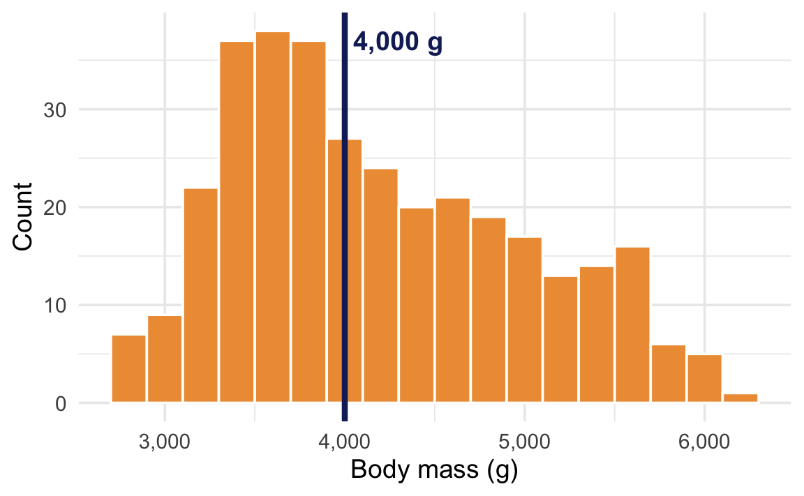
For this example, we’ll use the body mass of all penguins near Palmer Station, Antarctica. We want to know if the average body mass is different from 4,000 grams.

At first glance, it looks like most penguins are already roughly around 4,000 grams. Some are lighter, a lot are heavier, but 4,000 seems fairly reasonable.

We can look at this more officially. First, we’ll load some packages and check the official average weight:

library(tidyverse)
library(infer)
library(parameters)

penguins <- penguins |> drop_na(sex)

penguins |>
  summarize(avg_weight = mean(body_mass))

  avg_weight
1   4207.057

The sample mean is 4,207 g, which is a bit higher than our comparison value of 4,000 g. But is that difference real, or could it just be due to random chance?

Null hypothesis inference with {infer}

Step 1: Calculate \(\delta\)

The sample statistic we’re interested in is the mean body mass.

delta <- penguins |>
  specify(response = body_mass) |>
  calculate(stat = "mean")
delta

Response: body_mass (numeric)
# A tibble: 1 × 1
   stat
  <dbl>
1 4207.

The sample mean is 4,207 grams. We’re comparing this to μ₀ = 4,000 g, so the difference (δ) is 207 grams.

Step 2: Simulate null world

We create a null distribution by recentering our data around μ₀ = 4,000 g and then bootstrapping (resampling with replacement) from that shifted data. This creates a world where the true population mean is 4,000 g.

shuffled_data <- penguins |>
  specify(response = body_mass) |>
  hypothesize(null = "point", mu = 4000) |>
  generate(reps = 5000, type = "bootstrap")

Next we need to calculate the mean in each of these 5,000 resampled worlds:

null_world <- shuffled_data |>
  calculate(stat = "mean")
null_world

Response: body_mass (numeric)
Null Hypothesis: point
# A tibble: 5,000 × 2
   replicate  stat
       <int> <dbl>
 1         1 4010.
 2         2 4017.
 3         3 3939.
 4         4 3991.
 5         5 3946.
 6         6 3967.
 7         7 3965.
 8         8 4004.
 9         9 3986.
10        10 3930.
# ℹ 4,990 more rows

Here’s what this null world looks like:

null_world |>
  visualize()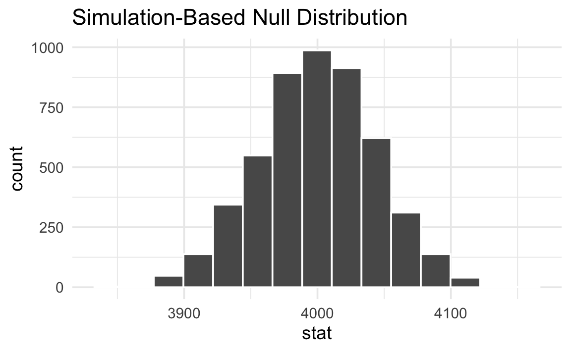

Notice that the null world is centered around 4,000 g—our comparison value—with variation reflecting what sample means would look like if the true mean really were 4,000 g.

Step 3: Put \(\delta\) in the null world

Next we put our observed sample mean inside that null world to see how comfortably it fits there.

null_world |>
  visualize() +
  shade_p_value(obs_stat = delta, direction = NULL)

That’s way out in the right tail. A sample mean of 4,207 g looks really unlikely in a world where the true mean is 4,000 g.

Step 4: p-value

We can quantify the probability of seeing that red line in a null world. This is a p-value—the probability of seeing a sample mean at least that far from μ₀ in a world where the true mean is 4,000 g.

null_world |>
  visualize() +
  shade_p_value(obs_stat = delta, direction = "two-sided")

p_value <- null_world |>
  get_p_value(obs_stat = delta, direction = "two-sided")

Warning: Please be cautious in reporting a p-value of 0. This result is an approximation based on the number of `reps` chosen in the `generate()` step.
ℹ See `get_p_value()` (`?infer::get_p_value()`) for more information.

p_value

# A tibble: 1 × 1
  p_value
    <dbl>
1       0

The p-value is < 0.001. This means that in a world where the true mean body mass is 4,000 g, there is a < 0.1% chance of seeing a sample mean at least as far from 4,000 as 4,207.

Step 5: Decision

Finally, we have to decide if the p-value meets an evidentiary standard or threshold that would provide us with enough evidence that we aren’t in the null world (or, in more statsy terms, enough evidence to reject the null hypothesis).

Using an α of 0.05, the p-value is < 0.001, which is less than 0.05. We have enough evidence to say that the average penguin body mass is statistically significantly different from 4,000 grams.

null_world |>
  visualize() +
  shade_p_value(obs_stat = delta, direction = "two-sided")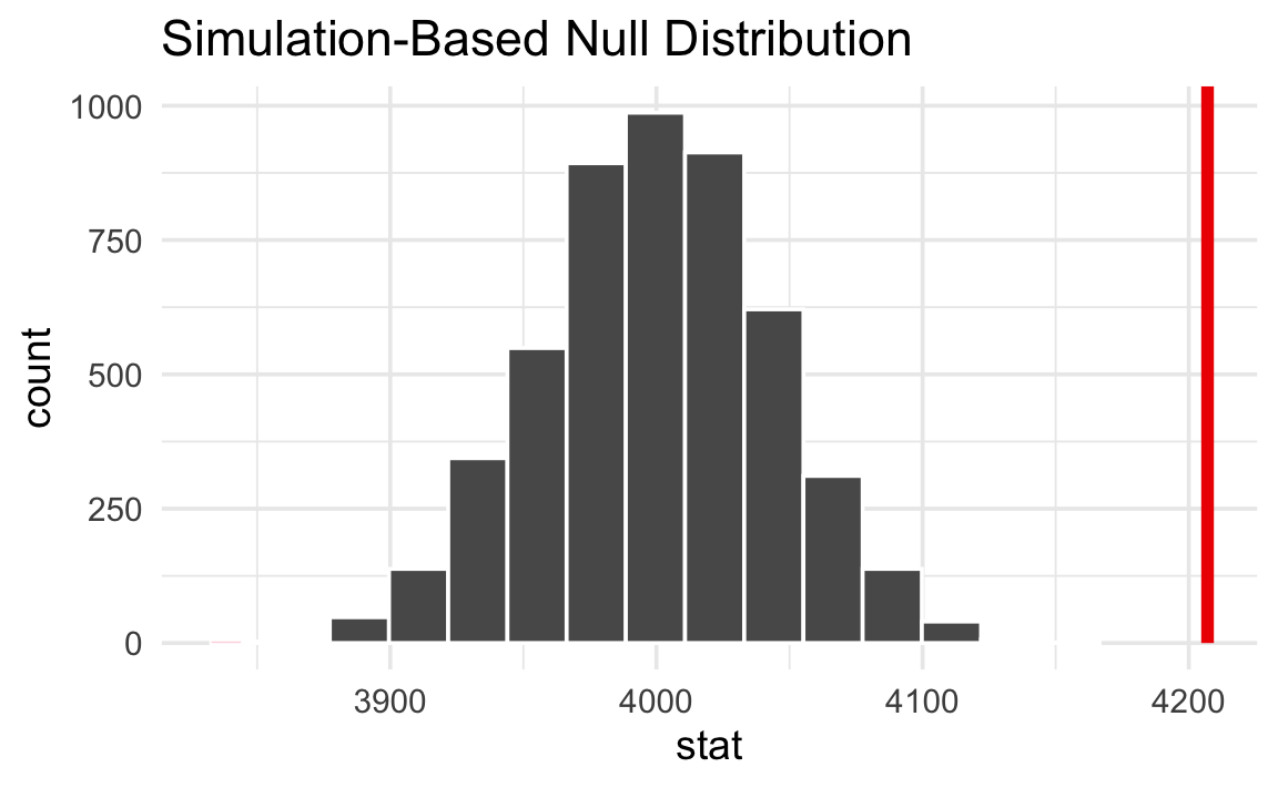

Null hypothesis inference with t.test()

In practice, most people do not simulate null worlds. Instead, they use a one-sample t-test, which approximates the null world mathematically using a t-distribution. The intuition is the same: a p-value is still the probability of seeing a sample mean at least that extreme in a world where the true mean is μ₀.

To test whether the average body mass differs from 4,000 g, we can use t.test() with mu = 4000:

t.test(penguins$body_mass, mu = 4000)

    One Sample t-test

data:  penguins$body_mass
t = 4.6925, df = 332, p-value = 3.952e-06
alternative hypothesis: true mean is not equal to 4000
95 percent confidence interval:
 4120.256 4293.858
sample estimates:
mean of x 
 4207.057 

The p-value is in that wall of text—it’s 3.952e-06, or 3.952 × 10⁻⁶, or 0.000003952. That’s really tiny. In a world where the average weight for all penguins is around 4,000 grams, it would be virtually impossible to see a difference as extreme as 4,207. We have enough evidence to declare that difference is statistically significant.

If you don’t like all that text output, you can feed the results of t.test() to the model_parameters() function from the {parameters} package:

t.test(penguins$body_mass, mu = 4000) |>
  model_parameters() |>
  display(caption = "")

Parameter	Mean	mu	Difference	95% CI	t(332)	p
Alternative hypothesis: true mean is not equal to 4000
body_mass	4207.06	4000	207.06	(4120.26, 4293.86)	4.69	< .001

Footnotes

1. Kind of—in common law systems, defendants are presumed innocent until proven guilty, so if there’s not enough evidence to prove guilt, they are innocent by definition.