Regression slope

Regression slope

◎◉○

Live simulation

jstat = require("jstat@1.9.6")

clrs = ({
  gold: "#f3d567",
  orange: "#ee9b43",
  coral: "#e74b47",
  crimson: "#b80422",
  navy: "#172767",
  teal: "#19798b",
  gray: "#4d4d4d"
})

// Simple OLS helper: returns { intercept, slope }
function ols(xvals, yvals) {
  const n = xvals.length;
  const mx = d3.mean(xvals);
  const my = d3.mean(yvals);
  let ssxy = 0, ssxx = 0;
  for (let i = 0; i < n; i++) {
    ssxy += (xvals[i] - mx) * (yvals[i] - my);
    ssxx += (xvals[i] - mx) * (xvals[i] - mx);
  }
  const slope = ssxy / ssxx;
  const intercept = my - slope * mx;
  return { intercept, slope };
}

function statLabel(value, textFn, dy, nullValues) {
  const extent = d3.extent([...nullValues, value]);
  const range = extent[1] - extent[0];
  const pos = range === 0 ? 0.5 :
    (value - extent[0]) / range;
  const textAnchor = pos > 0.82 ? "end" :
    pos < 0.18 ? "start" : "middle";
  const dx = textAnchor === "end" ? -10 :
    textAnchor === "start" ? 10 : 0;

  const common = {
    x: d => d, frameAnchor: "top", dy, dx,
    text: textFn,
    fontWeight: "bold", fontSize: 14,
    textAnchor, paintOrder: "stroke"
  };

  return [
    Plot.text([value], {
      ...common,
      stroke: "white", strokeWidth: 4, fill: "black"
    })
  ];
}

viewof sample_size = Inputs.range([30, 2000], {
  step: 10,
  value: 100,
  label: "Sample size:"
})

viewof slope_size = Inputs.range([-5, 5], {
  step: 0.1,
  value: 0.8,
  label: "Slope:"
})

viewof spread = Inputs.range([1, 15], {
  step: 1,
  value: 5,
  label: "Noise (σ):"
})

sample_data = {
  const data = [];
  for (let i = 0; i < sample_size; i++) {
    const x = Math.random() * 10;
    const y = 20 + slope_size * x +
      jstat.normal.sample(0, spread);
    data.push({ x, y });
  }
  return data;
}

obs_fit = ols(
  sample_data.map(d => d.x),
  sample_data.map(d => d.y)
)

Plot.plot({
  style: { fontSize: "13px"},
  marginLeft: 50,
  marginBottom: 45,
  width: 500,
  height: 350,
  x: { label: "Explanatory variable (x)", labelOffset: 35 },
  y: { label: "Outcome variable (y)" },
  marks: [
    Plot.dot(sample_data, {
      x: "x",
      y: "y",
      fill: clrs.navy,
      r: 3
    }),
    Plot.line(
      [
        { x: 0, y: obs_fit.intercept },
        { x: 10, y: obs_fit.intercept + obs_fit.slope * 10 }
      ],
      {
        x: "x",
        y: "y",
        stroke: clrs.crimson,
        strokeWidth: 2.5
      }
    )
  ]
})

Step 1: Calculate δ

The sample statistic (δ) is the regression slope—the estimated change in y for a one-unit increase in x.

model_stats = {
  const xvals = sample_data.map(d => d.x);
  const yvals = sample_data.map(d => d.y);
  const fit = ols(xvals, yvals);
  const n = xvals.length;

  // Residual standard error
  const mx = d3.mean(xvals);
  let ssxx = 0, sse = 0;
  for (let i = 0; i < n; i++) {
    const pred = fit.intercept + fit.slope * xvals[i];
    sse += (yvals[i] - pred) ** 2;
    ssxx += (xvals[i] - mx) ** 2;
  }
  const rse = Math.sqrt(sse / (n - 2));
  const se_slope = rse / Math.sqrt(ssxx);
  const se_intercept = rse *
    Math.sqrt(1 / n + mx * mx / ssxx);

  return {
    intercept: fit.intercept,
    slope: fit.slope,
    se_slope,
    se_intercept,
    ci_slope: [
      fit.slope - 1.96 * se_slope,
      fit.slope + 1.96 * se_slope
    ],
    ci_intercept: [
      fit.intercept - 1.96 * se_intercept,
      fit.intercept + 1.96 * se_intercept
    ]
  };
}

obs_stat = model_stats.slope

obs_stat_abs = Math.abs(obs_stat).toFixed(3)

The regression slope is .

html`<table class="table table-sm" style="max-width: 500px;">
  <thead>
    <tr>
      <th>Term</th>
      <th>Estimate</th>
      <th>95% CI</th>
    </tr>
  </thead>
  <tbody>
    <tr>
      <td>(Intercept)</td>
      <td>${model_stats.intercept.toFixed(3)}</td>
      <td>[${model_stats.ci_intercept[0].toFixed(3)}, ${model_stats.ci_intercept[1].toFixed(3)}]</td>
    </tr>
    <tr style="background-color: ${clrs.crimson}; color: white; font-weight: bold;">
      <td>x</td>
      <td>${model_stats.slope.toFixed(3)}</td>
      <td>[${model_stats.ci_slope[0].toFixed(3)}, ${model_stats.ci_slope[1].toFixed(3)}]</td>
    </tr>
  </tbody>
</table>`

Step 2: Simulate null world

We create a null distribution by shuffling (or “permuting” to use the official stats term) the values of x. This simulates a world where all the real, measured values of both x and y are still the same, but where the relationship between x and y doesn’t matter. This eliminates any association between x and y.

Think of this as being a world where there is no relationship between x and y. Importantly, this doesn’t mean that the slope is exactly 0. There is variation in the data, and that variation is reflected in the null world. What it means is that in the null world, the slope is 0 ± some amount.

Here’s what one shuffle looks like. Notice that the y values stay the same—only the x values get reassigned:

viewof reshuffle = Inputs.button("Reshuffle")

shuffle_preview = {
  reshuffle;
  const subset = sample_data.slice(0, 8);
  const xvals = subset.map(d => d.x);
  const shuffled_x = xvals.slice();
  for (let i = shuffled_x.length - 1; i > 0; i--) {
    const j = Math.floor(Math.random() * (i + 1));
    [shuffled_x[i], shuffled_x[j]] =
      [shuffled_x[j], shuffled_x[i]];
  }
  return {
    original: subset.map((d, i) => ({
      " ": i + 1,
      x: +d.x.toFixed(1),
      y: +d.y.toFixed(1)
    })),
    shuffled: subset.map((d, i) => ({
      " ": i + 1,
      x: +shuffled_x[i].toFixed(1),
      y: +d.y.toFixed(1)
    }))
  };
}

Original data

Inputs.table(shuffle_preview.original, {
  columns: [" ", "x", "y"],
  rows: 12,
  sort: false,
  select: false
})

Shuffled data

Inputs.table(shuffle_preview.shuffled, {
  columns: [" ", "x", "y"],
  rows: 12,
  sort: false,
  select: false
})

When we do this shuffle hundreds of times and fit a regression each time, we get a null distribution—a picture of what slopes look like in a world where x and y are unrelated.

Here’s what this null world looks like:

viewof n_reps = Inputs.range([100, 2000], {
  step: 100,
  value: 500,
  label: "Number of simulations:"
})

null_results = {
  const xvals = sample_data.map(d => d.x);
  const yvals = sample_data.map(d => d.y);
  const n = xvals.length;
  const stats = [];
  const lines = [];

  for (let r = 0; r < n_reps; r++) {
    // Fisher-Yates shuffle of x values
    const shuffled_x = xvals.slice();
    for (let i = n - 1; i > 0; i--) {
      const j = Math.floor(Math.random() * (i + 1));
      [shuffled_x[i], shuffled_x[j]] =
        [shuffled_x[j], shuffled_x[i]];
    }

    const fit = ols(shuffled_x, yvals);
    stats.push({ stat: fit.slope });
    lines.push({
      intercept: fit.intercept,
      slope: fit.slope
    });
  }
  return { stats, lines };
}

null_dist = null_results.stats

Plot.plot({
  style: { fontSize: "13px" },
  height: 300,
  width: 500,
  x: { label: "Slope" },
  y: { label: "Count" },
  marks: [
    Plot.rectY(
      null_dist,
      Plot.binX(
        { y: "count" },
        { x: "stat", fill: clrs.gray }
      )
    )
  ]
})

Here’s another way to see the null world slopes. Each thin line is a regression line for one of the simulated worlds where x and y are unrelated.

Plot.plot({
  style: { fontSize: "13px" },
  height: 300,
  width: 500,
  x: {
    label: "Explanatory variable (x)",
    domain: [0, 10]
  },
  y: { label: "Outcome variable (y)" },
  marks: [
    // Null world regression lines
    ...null_results.lines.map(l =>
      Plot.line(
        [
          { x: 0, y: l.intercept },
          { x: 10, y: l.intercept + l.slope * 10 }
        ],
        {
          x: "x",
          y: "y",
          stroke: "black",
          strokeWidth: 0.1,
          strokeOpacity: 0.3
        }
      )
    ),
    Plot.dot(sample_data, {
      x: "x",
      y: "y",
      fill: clrs.navy,
      fillOpacity: 0.7,
      r: 3
    })
  ]
})

Step 3: Put δ in the null world

Next we put δ inside that null world and see how comfortably it fits there.

Is it surprising to see the red line in this null world? Is the line way out to one of the sides, or is it near the middle with the rest of the null world?

Plot.plot({
  style: { fontSize: "13px" },
  height: 300,
  width: 500,
  x: { label: "Slope" },
  y: { label: "Count" },
  marks: [
    Plot.rectY(
      null_dist,
      Plot.binX(
        { y: "count" },
        { x: "stat", fill: clrs.gray }
      )
    ),
    Plot.ruleX([obs_stat], { stroke: "red", strokeWidth: 3 }),
    ...statLabel(obs_stat, d => `δ = ${d.toFixed(3)}`, 20,
      null_dist.map(d => d.stat))
  ]
})

Or alternatively, we can put the observed regression line from the actual data into the scatterplot with the null world regression lines. Is it surprising to see the red line in this null world?

Plot.plot({
  style: { fontSize: "13px" },
  height: 300,
  width: 500,
  x: {
    label: "Explanatory variable (x)",
    domain: [0, 10]
  },
  y: { label: "Outcome variable (y)" },
  marks: [
    ...null_results.lines.map(l =>
      Plot.line(
        [
          { x: 0, y: l.intercept },
          { x: 10, y: l.intercept + l.slope * 10 }
        ],
        {
          x: "x",
          y: "y",
          stroke: "black",
          strokeWidth: 0.1,
          strokeOpacity: 0.3
        }
      )
    ),
    Plot.dot(sample_data, {
      x: "x",
      y: "y",
      fill: clrs.navy,
      fillOpacity: 0.7,
      r: 3
    }),
    Plot.line(
      [
        { x: 0, y: obs_fit.intercept },
        { x: 10, y: obs_fit.intercept + obs_fit.slope * 10 }
      ],
      {
        x: "x",
        y: "y",
        stroke: "red",
        strokeWidth: 3
      }
    )
  ]
})

Step 4: p-value

We can actually quantify the probability of seeing that red line in a null world. This is a p-value—the probability of seeing a δ at least that extreme in a world where there’s no relationship between x and y.

p_value = {
  const abs_obs = Math.abs(obs_stat);
  const extreme = null_dist.filter(
    d => Math.abs(d.stat) >= abs_obs
  ).length;
  return extreme / null_dist.length;
}

p_value_clean = p_value === 0
  ? "< 0.001"
  : p_value.toFixed(3)

p_percent = p_value === 0
  ? "< 0.1%"
  : (p_value * 100).toFixed(1) + "%"

null_bins = {
  const values = null_dist.map(d => d.stat);
  const bin = d3.bin().thresholds(30);
  const bins = bin(values);
  const abs_obs = Math.abs(obs_stat);
  return bins.map(b => ({
    x0: b.x0,
    x1: b.x1,
    count: b.length,
    extreme: Math.abs((b.x0 + b.x1) / 2) >= abs_obs
  }));
}

Plot.plot({
  style: { fontSize: "13px" },
  height: 300,
  width: 500,
  x: { label: "Slope" },
  y: { label: "Count" },
  marks: [
    Plot.rectY(null_bins, {
      x1: "x0",
      x2: "x1",
      y: "count",
      fill: d => d.extreme ? clrs.coral + "aa" : clrs.gray,
      stroke: "white",
      strokeWidth: 0.5
    }),
    Plot.ruleX([obs_stat], { stroke: "red", strokeWidth: 3 }),
    ...statLabel(obs_stat, d => `δ = ${d.toFixed(3)}`, 20,
      null_dist.map(d => d.stat)),
    ...statLabel(obs_stat, () => `p = ${p_value_clean}`, 45,
      null_dist.map(d => d.stat))
  ]
})

// Also show the slope plot with observed line
Plot.plot({
  style: { fontSize: "13px" },
  height: 300,
  width: 500,
  x: {
    label: "Explanatory variable (x)",
    domain: [0, 10]
  },
  y: { label: "Outcome variable (y)" },
  marks: [
    ...null_results.lines.map(l =>
      Plot.line(
        [
          { x: 0, y: l.intercept },
          { x: 10, y: l.intercept + l.slope * 10 }
        ],
        {
          x: "x",
          y: "y",
          stroke: "black",
          strokeWidth: 0.1,
          strokeOpacity: 0.3
        }
      )
    ),
    Plot.dot(sample_data, {
      x: "x",
      y: "y",
      fill: clrs.navy,
      fillOpacity: 0.7,
      r: 3
    }),
    Plot.line(
      [
        { x: 0, y: obs_fit.intercept },
        { x: 10, y: obs_fit.intercept + obs_fit.slope * 10 }
      ],
      {
        x: "x",
        y: "y",
        stroke: "red",
        strokeWidth: 3
      }
    )
  ]
})

The p-value is

html`<p>This means that in a world where there is no relationship between x and y, there is a <strong>${p_percent}</strong> chance of seeing a slope of at least <strong>${obs_stat_abs}</strong></p>`

Step 5: Decision

Finally, we have to decide if the p-value meets an evidentiary standard or threshold that would provide us with enough evidence that we aren’t in the null world (or, in more statsy terms, enough evidence to reject the null hypothesis).

There are lots of possible thresholds. By convention, most people use a threshold (often shortened to α) of 0.05, or 5%. But that’s not required! You could have a lower standard with an α of 0.1 (10%), or a higher standard with an α of 0.01 (1%).

viewof alpha = Inputs.select([0.10, 0.05, 0.01], {
  label: "Significance threshold (α):",
  value: 0.05
})

{
  if (p_value < alpha) {
    return html`<div class="alert alert-success" role="alert">
      <h5 class="alert-heading">Statistically significant</h5>
      <p>The p-value is <strong>${p_value_clean}</strong> and our threshold for α is <strong>${alpha}</strong></p>
      <p>In a world where there is no relationship between x and y, the probability of seeing a slope of at least <strong>${obs_stat_abs}</strong> is <strong>${p_percent}</strong></p>
      <p>Since ${p_value_clean} is less than ${alpha}, we have enough evidence to say that the slope is <strong>statistically significant.</strong></p>
    </div>`;
  } else {
    return html`<div class="alert alert-warning" role="alert">
      <h5 class="alert-heading">Not statistically significant</h5>
      <p>The p-value is <strong>${p_value_clean}</strong> and our threshold for α is <strong>${alpha}</strong></p>
      <p>In a world where there is no relationship between x and y, the probability of seeing a slope of at least <strong>${obs_stat_abs}</strong> is <strong>${p_percent}</strong></p>
      <p>Since ${p_value_clean} is greater than ${alpha}, we don't have enough evidence to say that the slope doesn't come from the null world. The slope is thus <strong>not statistically significant.</strong></p>
      <hr>
      <p style="font-size: 0.9em;">This does <strong>not</strong> mean that there is no relationship between x and y! We just don't have enough evidence to judge if there's a relationship.</p>
    </div>`;
  }
}

Plot.plot({
  style: { fontSize: "13px" },
  height: 300,
  x: { label: "Slope" },
  y: { label: "Count" },
  marks: [
    Plot.rectY(null_bins, {
      x1: "x0",
      x2: "x1",
      y: "count",
      fill: d => d.extreme ? clrs.coral + "aa" : clrs.gray,
      stroke: "white",
      strokeWidth: 0.5
    }),
    Plot.ruleX([obs_stat], { stroke: "red", strokeWidth: 3 }),
    ...statLabel(obs_stat, d => `δ = ${d.toFixed(3)}`, 20,
      null_dist.map(d => d.stat)),
    ...statLabel(obs_stat, () => `p = ${p_value_clean}`, 45,
      null_dist.map(d => d.stat))
  ]
})

Plot.plot({
  style: { fontSize: "13px" },
  height: 300,
  x: {
    label: "Explanatory variable (x)",
    domain: [0, 10]
  },
  y: { label: "Outcome variable (y)" },
  marks: [
    ...null_results.lines.map(l =>
      Plot.line(
        [
          { x: 0, y: l.intercept },
          { x: 10, y: l.intercept + l.slope * 10 }
        ],
        {
          x: "x",
          y: "y",
          stroke: "black",
          strokeWidth: 0.1,
          strokeOpacity: 0.3
        }
      )
    ),
    Plot.dot(sample_data, {
      x: "x",
      y: "y",
      fill: clrs.navy,
      fillOpacity: 0.7,
      r: 3
    }),
    Plot.line(
      [
        { x: 0, y: obs_fit.intercept },
        { x: 10, y: obs_fit.intercept + obs_fit.slope * 10 }
      ],
      {
        x: "x",
        y: "y",
        stroke: "red",
        strokeWidth: 3
      }
    )
  ]
})

Evidentiary standards

When thinking about p-values and thresholds, I like to imagine myself as a judge or a member of a jury. Many legal systems around the world have formal evidentiary thresholds or standards of proof. If prosecutors provide evidence that meets a threshold (i.e. goes beyond a reasonable doubt, or shows evidence on a balance of probabilities), the judge or jury can rule guilty. If there’s not enough evidence to clear the standard or threshold, the judge or jury has to rule not guilty.

With p-values:

• If the probability of seeing an effect or difference (or δ) in a null world is less than 5% (or whatever the threshold is), we rule it statistically significant and say that the difference does not fit in that world. We’re pretty confident that it’s not zero.
• If the p-value is larger than the threshold, we do not have enough evidence to claim that δ doesn’t come from a world of where there’s no difference. We don’t know if it’s not zero.

Importantly, if the difference is not significant, that does not mean that there is no difference. It just means that we can’t detect one if there is. If a prosecutor doesn’t provide sufficient evidence to clear a standard or threshold, it does not mean that the defendant didn’t do whatever they’re charged with^†—it means that the judge or jury can’t detect guilt.

NoteDifferent evidentiary standards

Many legal systems have different levels of evidentiary standards:

• Standards of proof in most common law systems (juries):
  • Balance of probabilities (civil cases)
  • Beyond a reasonable doubt (criminal cases)
• Evidentiary thresholds in the United States (juries):
  • Preponderance of the evidence (civil cases)
  • Clear and convincing evidence (more important civil cases)
  • Beyond a reasonable doubt (criminal cases)
• Standards of proof in China (judges):
  • 高度盖然性 [gāo dù gài rán xìng] / highly probable (civil cases)
  • 证据确实充分 [zhèng jù què shí chōng fēn] / facts being clear and evidence being sufficient | the evidence is definite and sufficient (criminal cases)
• Levels of doubt in Sharia systems (judges):
  • غلبة الظن [ghalabat al-zann] / preponderance of assumption (ta’zir cases and family matters)
  • اليقين [yaqin] / certainty (hudud/qisas cases)
• Standard of proof in the International Criminal Court (judges):
  • Beyond reasonable doubt (genocide, crimes against humanity, or war crimes)

Flipper length and body mass

For this example, we want to know if flipper length predicts body mass in penguins near Palmer Station, Antarctica. Here’s a scatterplot of the relationship:

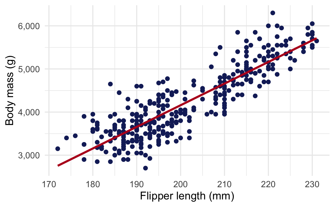
There’s a clear positive trend—penguins with longer flippers tend to be heavier. But is that relationship real, or could it just be due to random chance? Time for hypothesis testing!

First, we’ll load some packages:

library(tidyverse)
library(infer)
library(parameters)

penguins <- penguins |> drop_na(sex)

Null hypothesis inference with {infer}

Step 1: Calculate \(\delta\)

The sample statistic we’re interested in is the regression slope—the estimated change in body mass for a one-unit (1 mm) increase in flipper length.

delta <- penguins |>
  specify(body_mass ~ flipper_len) |>
  calculate(stat = "slope")
delta

Response: body_mass (numeric)
Explanatory: flipper_len (numeric)
# A tibble: 1 × 1
   stat
  <dbl>
1  50.2

The slope is 50.15, meaning that for every additional millimeter of flipper length, body mass increases by about 50.2 grams.

Step 2: Simulate null world

We create a null distribution by shuffling (or “permuting”) the flipper length values. This simulates a world where all the real, measured values of both flipper length and body mass are still the same, but where the relationship between them doesn’t matter. This eliminates any association between flipper length and body mass.

shuffled_data <- penguins |>
  specify(body_mass ~ flipper_len) |>
  hypothesize(null = "independence") |>
  generate(reps = 5000, type = "permute")

Next we fit a regression in each of these 5,000 shuffled worlds and extract the slope:

null_world <- shuffled_data |>
  calculate(stat = "slope")
null_world

Response: body_mass (numeric)
Explanatory: flipper_len (numeric)
Null Hypothesis: independence
# A tibble: 5,000 × 2
   replicate   stat
       <int>  <dbl>
 1         1  2.27 
 2         2  1.68 
 3         3  4.57 
 4         4  0.444
 5         5 -0.249
 6         6  3.07 
 7         7  2.17 
 8         8 -2.15 
 9         9 -3.02 
10        10 -2.78 
# ℹ 4,990 more rows

Here’s what this null world looks like:

null_world |>
  visualize()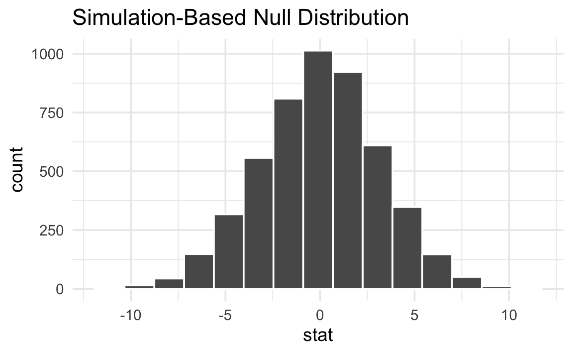

Notice that the slopes are centered around 0, reflecting a world where flipper length and body mass are unrelated.

Step 3: Put \(\delta\) in the null world

Next we put δ inside that null world to see how comfortably it fits there.

null_world |>
  visualize() +
  shade_p_value(obs_stat = delta, direction = NULL)

That’s way far to the right and doesn’t look likely at all. A slope of 50.15 is really unlikely in a world where flipper length and body mass are unrelated.

Step 4: p-value

We can quantify the probability of seeing that red line in a null world. This is a p-value—the probability of seeing a slope at least that extreme in a world where there’s no relationship between flipper length and body mass.

null_world |>
  visualize() +
  shade_p_value(obs_stat = delta, direction = "two-sided")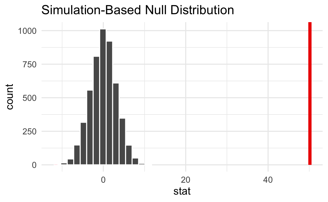

p_value <- null_world |>
  get_p_value(obs_stat = delta, direction = "two-sided")

Warning: Please be cautious in reporting a p-value of 0. This result is an approximation based on the number of `reps` chosen in the `generate()` step.
ℹ See `get_p_value()` (`?infer::get_p_value()`) for more information.

p_value

# A tibble: 1 × 1
  p_value
    <dbl>
1       0

The p-value is < 0.001. This means that in a world where flipper length has no relationship to body mass, there is a < 0.1% chance of seeing a slope at least as extreme as 50.15.

Step 5: Decision

Finally, we have to decide if the p-value meets an evidentiary standard or threshold that would provide us with enough evidence that we aren’t in the null world (or, in more statsy terms, enough evidence to reject the null hypothesis).

Using an α of 0.05, the p-value is < 0.001, which is less than 0.05. We have enough evidence to say that the relationship between flipper length and body mass is statistically significant.

null_world |>
  visualize() +
  shade_p_value(obs_stat = delta, direction = "two-sided")

Null hypothesis inference with lm()

In practice, most people do not simulate null worlds. Instead, they fit a regression model with lm(), which uses a t-distribution to approximate the null world mathematically and test whether each coefficient is different from 0. The intuition is the same: a p-value is still the probability of seeing a slope at least that extreme in a world where the true slope is 0.

model <- lm(body_mass ~ flipper_len, data = penguins)
summary(model)

Call:
lm(formula = body_mass ~ flipper_len, data = penguins)

Residuals:
     Min       1Q   Median       3Q      Max 
-1057.33  -259.79   -12.24   242.97  1293.89 

Coefficients:
            Estimate Std. Error t value Pr(>|t|)    
(Intercept) -5872.09     310.29  -18.93   <2e-16 ***
flipper_len    50.15       1.54   32.56   <2e-16 ***
---
Signif. codes:  0 '***' 0.001 '**' 0.01 '*' 0.05 '.' 0.1 ' ' 1

Residual standard error: 393.3 on 331 degrees of freedom
Multiple R-squared:  0.7621,    Adjusted R-squared:  0.7614 
F-statistic:  1060 on 1 and 331 DF,  p-value: < 2.2e-16

Buried in that output is the p-value for the flipper_len coefficient: p < 2.2e-16, or p < 2.2 × 10⁻¹⁶. That’s really tiny. In a world where flipper length had no relationship with body mass, it would be virtually impossible to see a slope as extreme as 50.15. We have enough evidence to declare that the relationship is statistically significant.

If you don’t like all that text output, you can feed the model to the model_parameters() function from the {parameters} package:

model |>
  model_parameters() |>
  display(caption = "")

Parameter	Coefficient	SE	95% CI	t(331)	p
(Intercept)	-5872.09	310.29	(-6482.47, -5261.71)	-18.92	< .001
flipper len	50.15	1.54	(47.12, 53.18)	32.56	< .001

Footnotes

1. Kind of—in common law systems, defendants are presumed innocent until proven guilty, so if there’s not enough evidence to prove guilt, they are innocent by definition.